People tend to think first of Henry's Law, which suggests a fixed partition of a solute (including gas) between two phases. This is a material property, and refers to equilibrium, which does not apply to CO2 in air/sea. It applies even less to the land sink, which is quite important.
In this note, I will show that the constancy, perversely, depends on the dynamics, and is a result of the near exponential increase in CO2 emissions. This effect is mostly independent of the actual mechanism for the sinks. It is really a consequence of linearity with exponential increase.
Since this post is something of a math proof, here is a TOC:
- Cumulative plotting
- Exponential emissions
- Steady observed airborne fraction
- Linearity and superposition.
- Airborne fraction invariance
- Airborne fraction if emissions growth is not exponential
Cumulative plotting
People usually discuss airborne fraction as a ratio of annual increment of mass of CO2 in air to the increment injected. For example, the AR4 shows Fig 7.4.1: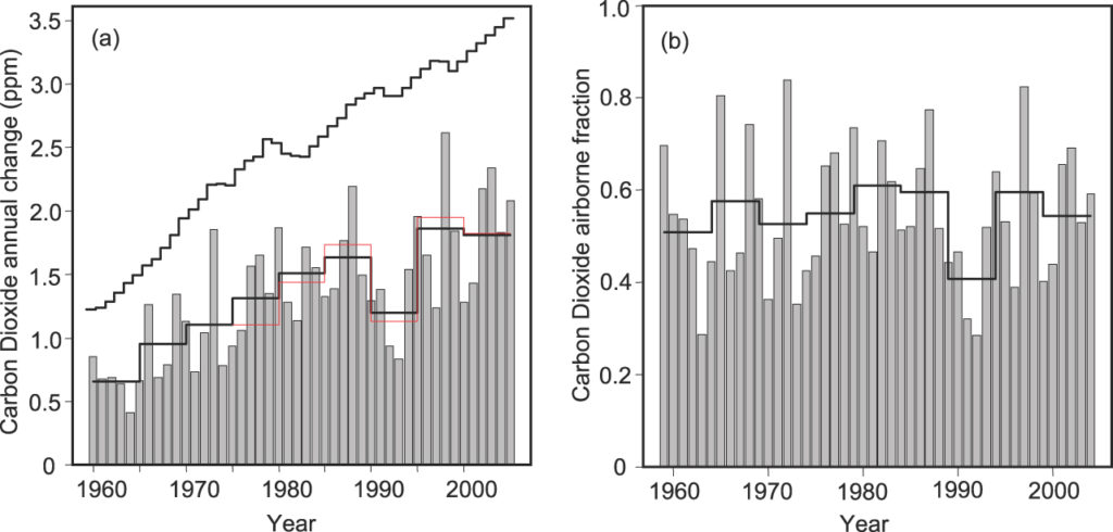
On that basis, there are papers here and here, which suggest the fraction may be increasing.
I think that method of calculation loses information about the CO2 buildup. Ppmv CO2 is measured as a succession of states. The differences by year are quite noisy, but the noise cancels. When you measure the state in 2015, that is unaffected by noise in previous measures. With cumulative emissions, this is not true. Noise in annual emissions accumulates, with no corrective state measure.
The conventional AF uses the annual differences of CO2 ppm, and loses the benefits of stabilizing state measure. It might be said that this does not matter so much, because it is divided by emissions, which don't have a state measure. But emissions are, or should be, more accurately determined. They are economic statistics, compiled by an army of accountants.
Exponential emissions
I'll be talking more about the exponential increase in emissions. The usual way to illustrate that is with a log plot. Here are the cumulative total emissions as a function of time, up to 2011: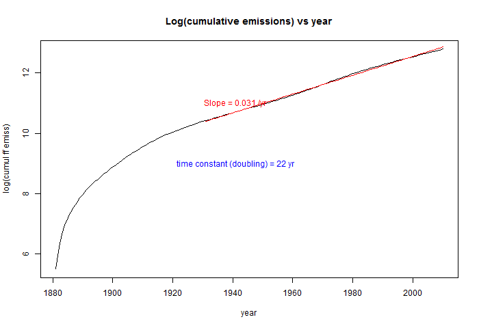
It's very close to exponential from about 1930 onward, with doubling time 22 years. So the annual increments must follow a similar exponential, with more noise. One might ask - should I have plotted the increments. I don't think so - I'll be using integrals of the emission rate.
Steady observed airborne fraction
So I'll show the more stable measure. But first I note that there are actually two airborne fractions quoted. One is the ratio of CO2 in air to total emissions, including land use. This comes to about 0.44. The other is the ratio to fossil fuel (and cement) emissions alone, which is about 0.55. I plotted both here, and both arre stable; I'll refer to the total emissions in this post. The plot showing stability is here: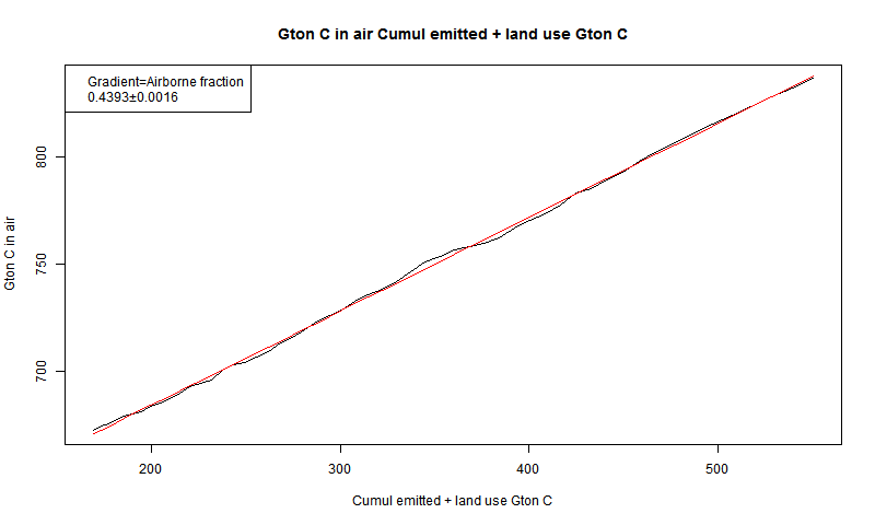
I have tracked the cumulative emissions from about 180 to 530 Gtons. If you go back to early times, the line does start to waver.
Linearity and superposition.
I discussed the application of the Bern model here. That model supposes a impulse response function (IRF), and that is the basis for my theory here. The idea of an IRF is that each puff of CO2 emitted has a time course in the atmosphere, which is the same for puffs emitted at different times (relative to emission), and the different puffs to not interfere with each other. These are widely applicable assumptions, and depend little on the detail of the absorption mechanism. The practical consequence is that you can represent the CO2 in the air at any time as the added effect of all the puffs:M(t) = ∫ E(t-τ) F(τ) dτ
where E is the emission rate, F the IRF, M the mass of CO2, and the integral goes from -∞ to 0. It says that if E(t-τ) dτ was emitted time τ ago, a fraction F(τ will now remain, and the total is the sum of these fractions.
Airborne fraction invariance
So suppose exponential growth E(t)=a*exp(b*t). ThenM(t) = a*∫ exp(b*(t-τ)) F(τ) dτ= a*exp(b*t)∫ exp(-b*τ) F(τ) dτ ...again, the integral goes from -∞ to 0
Now the integral does not depend on t. The denominator of the airborne fraction is just the same expression with F=1 - ie as if no decay happened at all. Then for all t, the ratio is
AF = ∫ exp(-b*τ) F(τ) dτ/∫ exp(-b*τ) dτ = b*∫ exp(-b*τ) F(τ) dτ
This is actually just minus the Laplace Transform of the derivative of F at b. But it is independent of t, for any (reasonable) F.
Airborne fraction if emissions growth is not exponential
Well, first as seen above, it actually isn't really exponential before about 1930. But these are integrals - that part of the curve makes in modern times a very small contribution. But what if it changed in future?Suppose emissions slowed. You'd expect that with more time to be absorbed, the AF would diminish. In terms of these integrals, we have the laplace transform of a diminishing function F divided by the transform of 1. Both will increase, but the transform of 1 will rise faster (behaviour at ∞) so again, the AF will diminish. Emissions rising faster than the current exponential would see the AF increase.
The paper of Knorr cited above, and some others, suggest the AF may be increasing. If so, this would be because of a divergence from linearity, probably caused by saturation of sinks. This is worrying from an AGW point of view; the relatively low AF has been a mitigator. But there is no sign of an increase in the cumulative plots.


One minor note: in your previous post about the Bern model, you weren't really discussing the Bern model, but rather the approximation to the Bern model. The Bern model itself is a more complex box-model approach to the carbon cycle (see, for example, this 1996 description: http://www.climate.unibe.ch/~joos/model_description/model_description.html)
ReplyDeleteBut yes, I agree that the relatively constant AF is not a physical feature of the earth system, but rather a coincidence based on having an emissions growth that is just fast enough. I believe that for AR5, there was more discussion of the AF in the proposed draft, but after some critiques, the discussion was pared down in the final version (correctly, in my opinion)
-MMM
Yes, I agree that I was really dealing with an impulse response function extracted from the Bern Model. It enabled me to investigate whether the invariance of AF held there.
DeleteNick, I did the Green's function (i.e. impulse response) approach for CO2 sequestration a few years ago, already published here
Deletehttps://books.google.com/books?id=oY2ZPn5EOTQC
Physicists quickly recognize that the Bern Model is just an approximation to to the solution to the diffusion equation. And to simplify the math, superstatistics or MaxEnt is applied to model the various diffusional pathways.
So the math that I have is an analytical closed-form solution to a "box" diffusion model that can normally only be calculated numerically.
And of course, since it is also diffusion, this approach can be used to model thermal uptake in the ocean
http://theoilconundrum.blogspot.com/2013/03/ocean-heat-content-model.html
Climate science is lagging in being able to model the physics via these simplified formulations.
Paul,
DeleteI think you're referring to about p 594 in your book. Unfortunately, for me that was in the not visible part. I did see some later convolution treatment.
And yes, that's the basis of Bern model. I'm mainly focussing here on the particular property that exponential rise of emissions implies steady AF.
The book is located elsewhere. Yes paginated 594 or page 604 of the PDF file:
Deletehttp://daina.com/published/TheOilConundrum.pdf
Steady air-borne fraction is a result of the random walk diffusion, which is a kinetic process.
Paul,
DeleteThanks, I read it. Dispersion in the sea is a diffusive process, but there isn't just one D - it's highly variable with space. And the land sink isn't obviously subject to a diffusion equation. The thing about exponentials (Bern) is that they provide fairly simple basis functions for representing a diminishing IRF. Error functions would do much the same.
What I'm trying to show here is that the apparent constancy results not from the form of the IRF - diffusive or whatever, but the form of the emissions rise (exponential).
Bravo, Nick! An elegant and concise explanation of the rather surprising observation of a constant AF over recent decades.
Delete"Dispersion in the sea is a diffusive process, but there isn't just one D - it's highly variable with space. "
DeleteThat's why I call it Dispersive Diffusion -- a range of D values are incorporated in my model. Because of this explicitly modeled range of values, it works much better than what is currently available. Yes, you can say that D varies spatially, but that's a second-order effect compared to incorporating the variability in D at all.
The beauty is that the variability is set via the MaxEnt principle, which provides maximum uncertainty given that all that is known is the overall mean diffusivity D.
All the rest of what you are doing is also in the book, because that is what an impulse response function is typically used for -- the impulse is convolved with the forcing function, in this case carbon emissions. The result is used to determine the sequestered amount and the airborne amount. I am not sure why you didn't use the term convolution when you are describing this in your mathematics. The term is certainly widely known as you can Google "convolution" "co2" "sequestration" and see what others have done before. The new thing is having a simple yet expressively powerful impulse response function, which is what I pitched in.
Interesting. What about the issue that the ability of the ocean to uptake CO2 decreases at higher temperature and at higher CO2 concentrations, and also whether or not we'll see a decrease in the ability of the biosphere to continue taking up the same fraction of the CO2? I thought there were nutrient issues with the uptake of CO2 by the biosphere?
ReplyDeleteATTP,
DeleteMy contention here is that constant AF follows from a time-invriant linear transfer function and an exponential driver (emissions). To some extent, temperature reducing CO2 solubility would have a component that is just folded into the apparent response function. But yes, any non-linear effect of that, or biosphere response, could cause a variation in AF, even with exponential emissions.
Chemical reaction is also potentially non-linear. Most CO2 reacts to form a carbonate species, but as long as the carbonates are in excess, so have little proportional change, it just works as an apparent increased solubility. But if CO3-- gets significantly depleted, that would have non-linear effect.
Okay, thanks.
DeleteNick,
ReplyDeleteI have come to the conclusion that if emissions were held constant for 30 years then the airborne fraction would reduce to aero. In other words if the world held emissions constant at say 30GT CO2/y then sinks would increase to balance emissions. Thereafter CO2 levels would remain at say 450ppm indefinitely so long as emissions remained constant.
I claim that after stabilisation of emissions, carbon sinks would follow a (1/2)^n increase until balance is reached, where n = 1-10years. Yes we would be stuck with CO2 at 450ppm indefinitely and say 2C warming, at least until we found another energy source.
Clive
Clive,
DeleteI guess you're referring to your post here. Well, I agree, as in this post, that it is AF is dynamic, and if emissions stabilise, it would go down. And yes, at some stage, if the sinks were infinite (really, of zero impedance), it could go to zero. But that is a big assumption.
Thanks Nick,
DeleteUnder long enough time scales the sinks are infinite. You only have to look at Limestone mountains to see that. However it may buy us enough time to fix the energy problem properly. Short term ocean acidification in the surface zone is another problem, but mixing with deep ocean is faster than people think.
Clive, the problem with the CO2 emissions is that for the sum of atmosphere, ocean, and biosphere there is almost no sink at all.
ReplyDeleteSo the current 'sink' from perspective of the atmosphere is only a redistribution of the carbon from the atmosphere to the ocean and the biosphere.
If one wish to stabilize the atmospheric CO2 level, there is the need to stabilize the sum of the carbon content of atmosphere, ocean and biosphere too.
If one wish to stabilize the atmospheric CO2 level at about 450 ppm, there must be an emission equal to the increase of the small sink of the sum of atmosphere, ocean, and biosphere compared to the natural level. Then the carbon content of the atmosphere, ocean, and biosphere will remain constant indefinitely and the atmospheric CO2 level will remain constant too (except for a redistribution between atmosphere, ocean, and biosphere). The CO2 emissions needed to hold the carbon content of the atmosphere, ocean, and biosphere and the atmospheric CO2 level constant at about 450 ppm is 0.078 GT CO2/yr.
A constant emission at 30 GT CO2/yr would lead to a continuous rising of the sum of the carbon content of the atmosphere, ocean, and biosphere and the atmospheric CO2 level until we ran out of fossil fuels or atmospheric oxygen (depending on the size of the remaining fossil fuels, atmospheric oxygen content is well known).
Uli,
DeleteWhat your saying is that the only long term sink of the combined atmosphere-ocean-biosphere is the slow accumulation of sediments on the ocean floor. These come from rock weathering and phytoplankton etc. But even these are not sinks for ever as slowly sedimentary rock gets swept down subduction zones to emit CO2 to the atmosphere again in Volcanoes and mid ocean expansion zones.
What I am talking about is just the rebalancing of anthropogenic CO2 between ocean atmosphere and biosphere. What we are doing is bad but not catastrophic. Super-volcanoes were probably far worse but the carbon cycle coped and so it will this time.
To avoid making matters worse we have to fix emissions so that the natural rebalancing has a chance to work.
Have to at least listen to what Clive says. Can't help but point out that the Bern model is a crude heuristic -- especially in terms of not being able to describe what should be a rather obvious dispersive diffusional model of CO2 sequestering.
DeleteI can't help the fact that I did detailed dopant diffusion models while I worked at IBM Watson and so can easily understand how the Bern model is a heuristic stab at the real thing.
As far as inferring long-term implications, I don't really think I should until the scientists start producing a better statistical physics-based impulse response (i.e. Green's function) than the junk Bern model. No one in the semiconductor industry would ever use a diffusional model that crudely constructed.
Clive, the slow accumulation of sediments and the burial of organic carbon too. And yes they are not forever but for a very long time, but many millions of years as the age of these sediments shows.
DeleteI think your (1/2)^n assumption is wrong, because is neglects the increase of the carbon content in the sink.
Think about what would happen if we not hold the emissions constant at current level, but would reduce it in less than one year to the level of the current atmospheric sinks (to about 17-18 GT CO2/yr) and held it at this rate constant indefinitely.
The rise of the atmospheric carbon content, and therefor the rise of the CO2 level would come to a sudden stop, because the emissions and sinks where equal. But it does not come to a steady state for ever. The carbon content of the sinks will continue to increase. And so will partial pressure difference between the atmosphere and the sink, which ensures the uptake of the sink, decrease, because the partial pressure of CO2 in the atmosphere is constant for a while, but the lower partial pressure in the sink increases due to the continued carbon uptake of the sink. As the uptake of the sinks from the atmosphere decrease, we would either need to lower the emissions further to hold the atmospheric CO2 level constant, or the atmospheric CO2 level starts to increase again.
So a stabilization of the atmospheric carbon content needs a stabilization of the ocean carbon content too.
You can also think about what would happen, if we would the emit the whole CO2 not to the atmosphere but to the ocean. How would the carbon content of the ocean and the atmosphere change then?
@whut, I think the main question for the long term is: How does the equilibrium distribution of the carbon content of the atmosphere, ocean and biosphere change, when the total carbon content of the atmosphere, ocean and biosphere changes?
So suppose exponential growth E(t)=a*exp(b*t).
ReplyDelete....
AF = ∫ exp(-b*τ) F(τ) dτ/∫ exp(-b*τ) dτ = b*∫ exp(-b*τ) F(τ) dτ
This is an elegant demonstration why AF is nearly constant. Neat.
Now if we estimate E(t) as about 2% per year growth and assume F(τ) is a single exponential decay doesn't this allow an empirical estimation of the time constant of F(τ) ?
ie the residence time of CO2 in the atmosphere?
regards, Greg.
2% doubles in 35 and gives b=50y unless I'm mistaken.
DeleteAF = b*∫ exp(-b*τ) F(τ) dτ
F(τ)= exp(-b2*τ) is now soluable, no?
Greg,
DeleteThanks. b there would be 1/50. But yes, as you've posed it, AF=b/(b+b2) which is easily solved.
I did a calc here (see earlier comment, of which this is correction). It gives AF=.488, but ATTP downthread showed that with AR5 numbers it is about 0.56. Which is right for total emissions (incl land use). I guess that's no surprise; the Bern model would have been constructed to get that right.
Sorry, it was Clive with the AR5 numbers.
DeleteGoodman is another one of those dudes that apparently hasn't been trained in physics. Diffusion gives a fat-tail response so you can't use a damped exponential as an impulse response function.
DeleteAll this was discussed up-thread last year.
But better yet. Here is a simple explanation for the value of 0.5. Diffusion is a random walk model. CO2 sequestration is a 1-D random walk of molecules into the ocean. Once a CO2 molecule enters the ocean, it has a 50% chance of going deeper and a 50% chance of popping back out. That's 50% = 0.5. Nuff said. Or set up a detailed slab calculation and you will find the same thing. Why do people make this so hard?
"I guess that's no surprise; the Bern model would have been constructed to get that right."
DeleteI thought that the Bern model was semi-empirical based on trace element studies.
Indeed it does look like the multiple parameters ( seven ) of the Bern model have been retweaked since AR4. This is typically the problem with climatology: too many poorly constrained variables and unrealistic claims of certainty about the resulting values.
I don't see how we can have much confidence in a0 and the "179y" parameters on the basis of the length of evidence available. Sadly they are the ones which are the most important for estimating how long CO2 will remain in the atmosphere and what the effects of any particular emissions scenario will be.
The idea is a mix of diffusivities. I have one way to solve this but there are others
Deletehttps://arxiv.org/abs/1611.06202 -- Brownian yet non-Gaussian diffusion: from superstatistics to subordination of diffusing diffusivities
To do earth sciences effectively you have to know when to apply stochastic models and when to apply deterministic models.
"This is typically the problem with climatology: too many poorly constrained variables and unrealistic claims of certainty about the resulting values."
ReplyDeleteCould you quote those "claims of certainty" about the parameters?
I don't think there are any, or that it matters. Expressing an impulse response function as a sum of exponentials does yield poorly constrained parameters. The reason is that the exponentials are far from orthogonal, and different parameter combinations can give the same result. It is that same resulting IRF that matters.
The BERN model is a semi-empirical model tuned to match observed carbon cycle behaviour. That would include AF.
Joos et al 2013:
ReplyDeletewww.atmos-chem-phys.net/13/2793/2013/acp-13-2793-2013.pdf
"For a 100 Gt-C emission pulse added to a constant CO2 concentration of 389 ppm, 25 ± 9 % Ocean is still found in the atmosphere after 1000 yr"
That is essentially saying a0=0.25 ± 9 % , though that probably is drawn from the distribution of group of models they are looking at rather than anything which could be regarded as an experimental uncertainty.
The link to joos upthread has just vanished on the "new site" at U. Bern, although google still has it.
The description includes land sinks; different ocean boxes including a high latitude, well-mixed, ocean sink so it is not simply a four term exponential approximation to a diffusion model.
http://clivebest.com/blog/wp-content/uploads/2016/11/Fraction-reatined-AR4.png
Though AF seems essentially level over the record, there is quite significant variability including a notable dip in 60s and 70s and around the Mt Pinatubo cooling and 1998 El Nino. There should be some useful empirical cross-checks to be gained from looking at that variation in AF as well as it's long term constancy.
Greg.
oops that should be : high latitude, well-mixed, DEEP ocean sink
Deletethis presumably reflects that high latitudes are dominated by THC and not diffusion.
Greg,
ReplyDelete....25±9% remains in the atmosphere, while " the ocean has absorbed 59 ± 12 % and the land the remainder (16 ± 14 %)".
I presume there errors are correlated, because If not then Land could be 30% and the Ocean could be 70% !
Richard Betts recently tweeted about a paper from 1972 on "Man-made Carbon Dioxide and the 'Greenhouse' effect" by J. S. Sawyer, which contained:
ReplyDelete"Industrial development has recently been proceeding at an increasing rate so that the output of man-made carbon dioxide has been increasing mode or less exponentially. So long as the carbon dioxide output continues to increase exponentially, it is reasonable to assume that about the same proportion as at present (about half) will remain in the atmosphere and about the same will go into the other reservoirs."
which suggests that the dependence of the approximately constant airborne fraction on the exponential rise in anthropogenic emissions is well understood by carbon cycle researchers, and has been for some times. However it is probably one of those things so obvious to those working on the topic that it goes unsaid in the journal papers, so it is good to have accessible explanations!
I demonstrated a similar result using a much more basic (simple one-box) carbon cycle model in my paper
Gavin C. Cawley, On the atmospheric residence time of anthropogenically sourced carbon dioxide, Energy & Fuels, volume 25, number 11, pages 5503–5513, September 2011. (preprint)
But obviously the impulse-response-of-the-BERN-model-model give far more reliable quantative projections, so this is article is a really useful resource.